Effective Data Communication With {ggplot2}
Part II - Putting theory into practice
2024-06-13
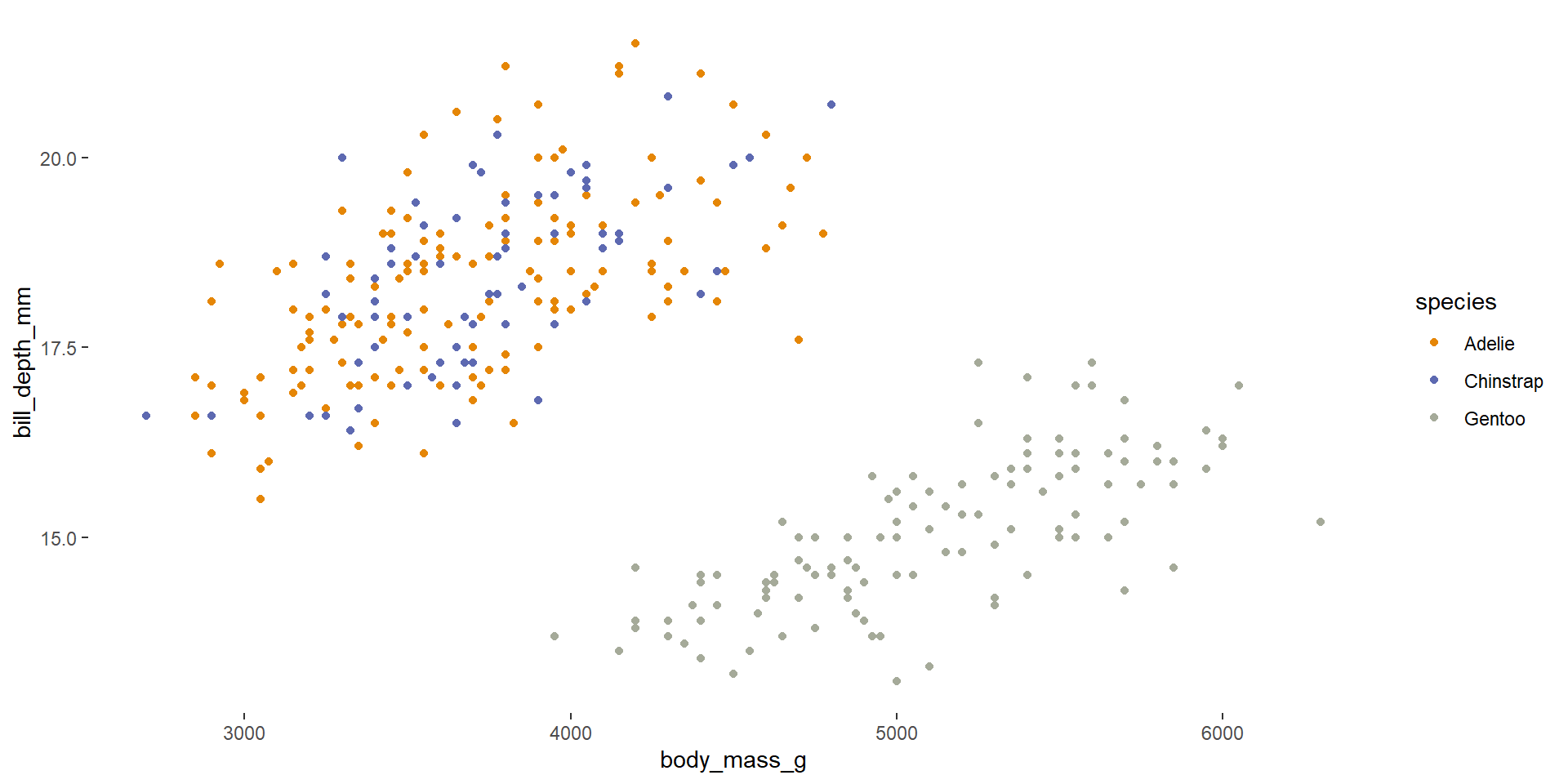
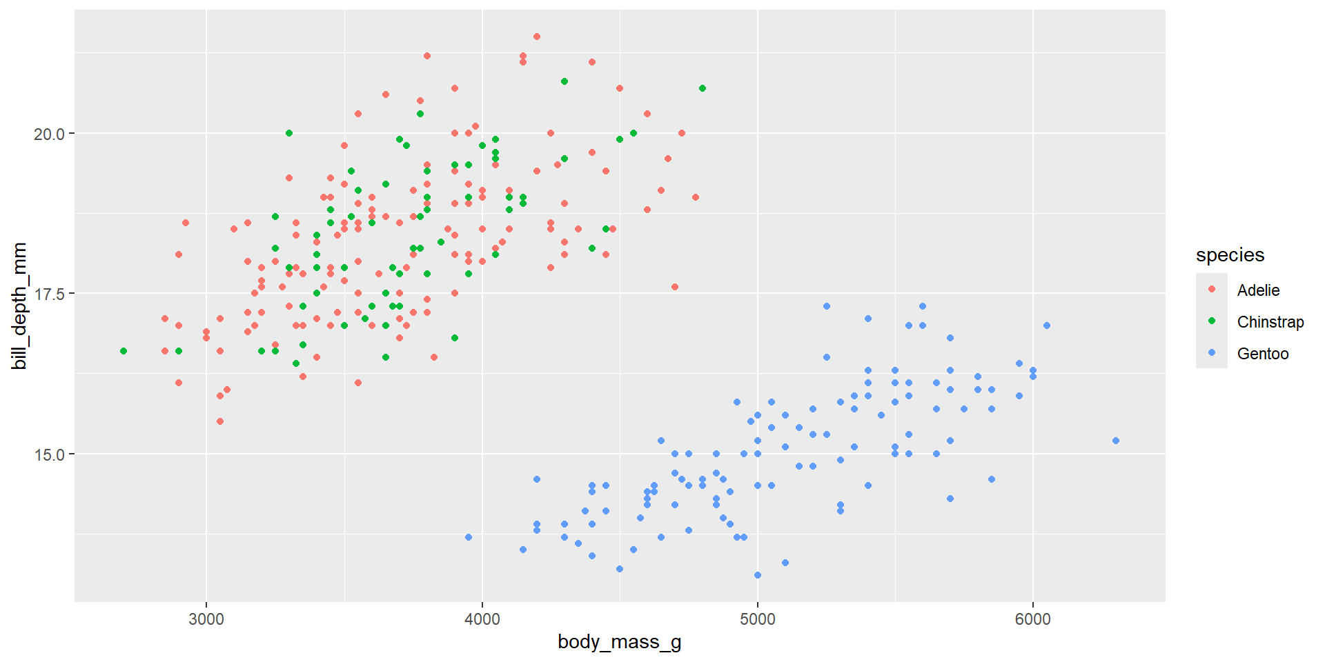
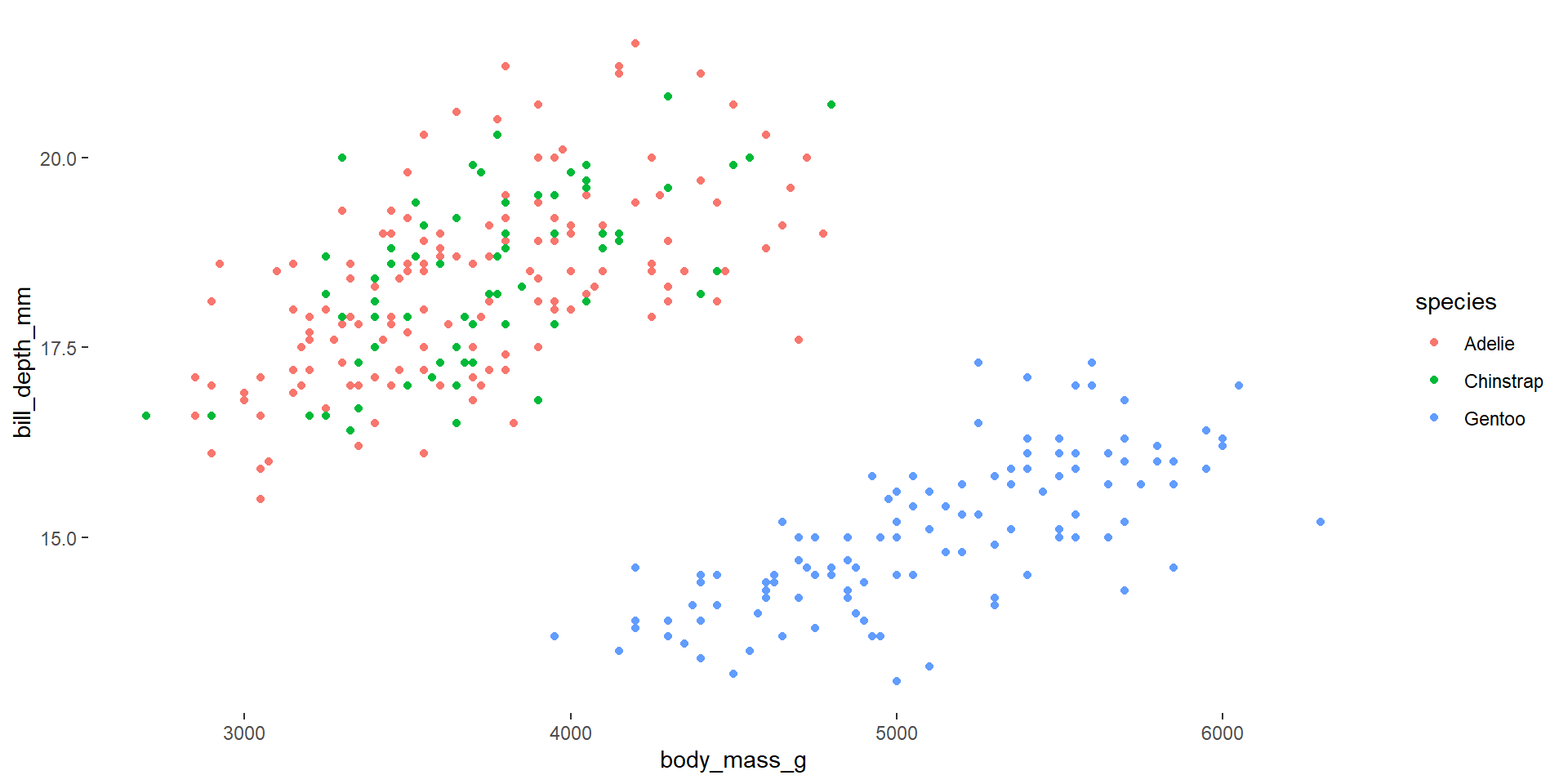
The {ggplot2} default
{theme_*}
{theme_*}
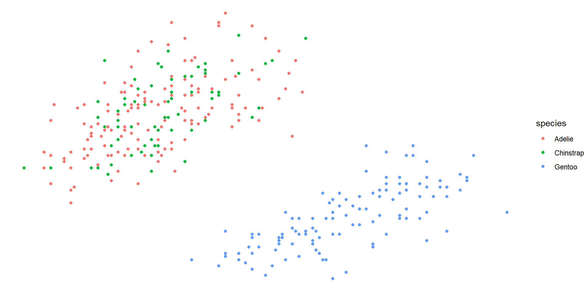
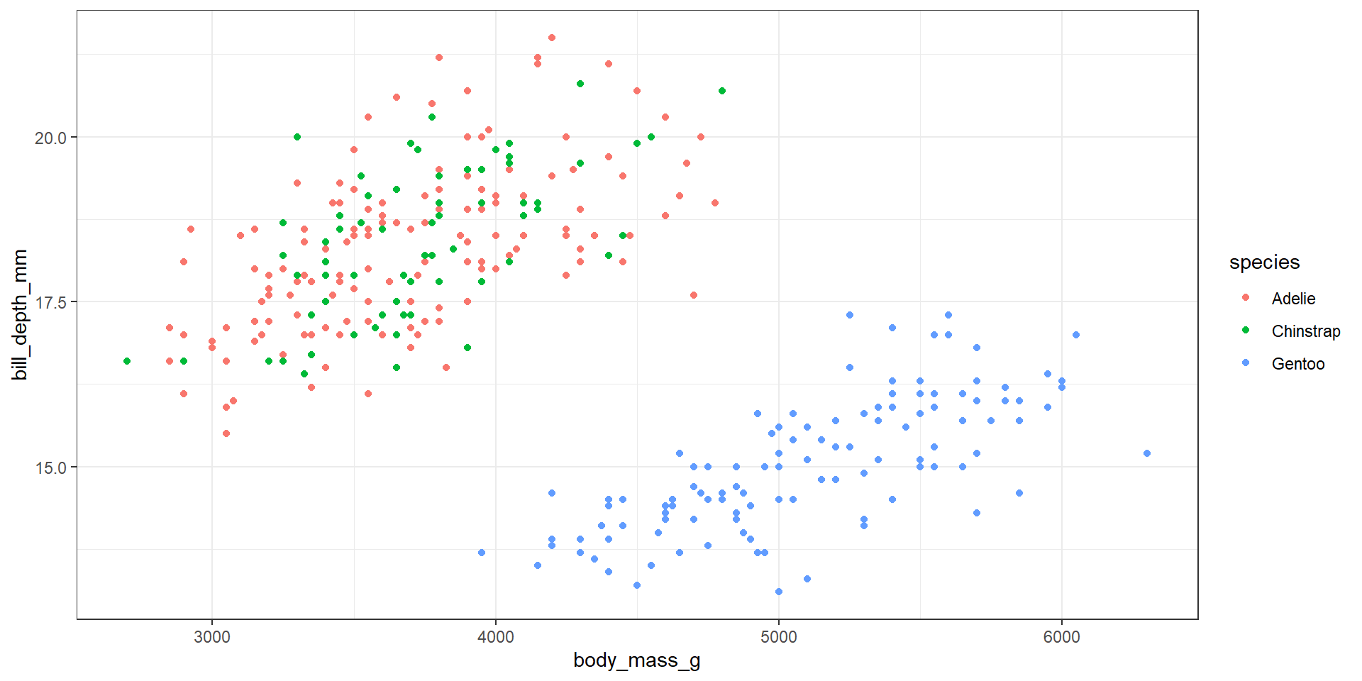
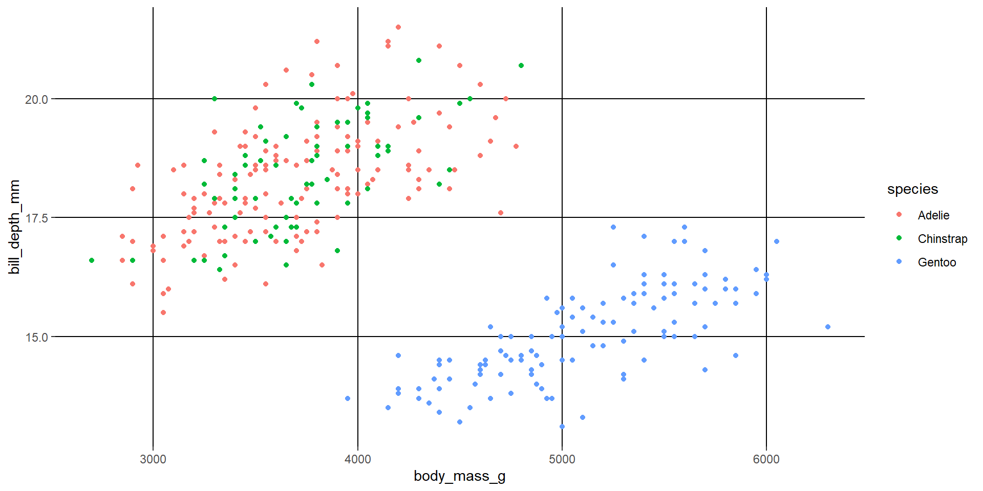
Remove the background panel
Re-add grid lines
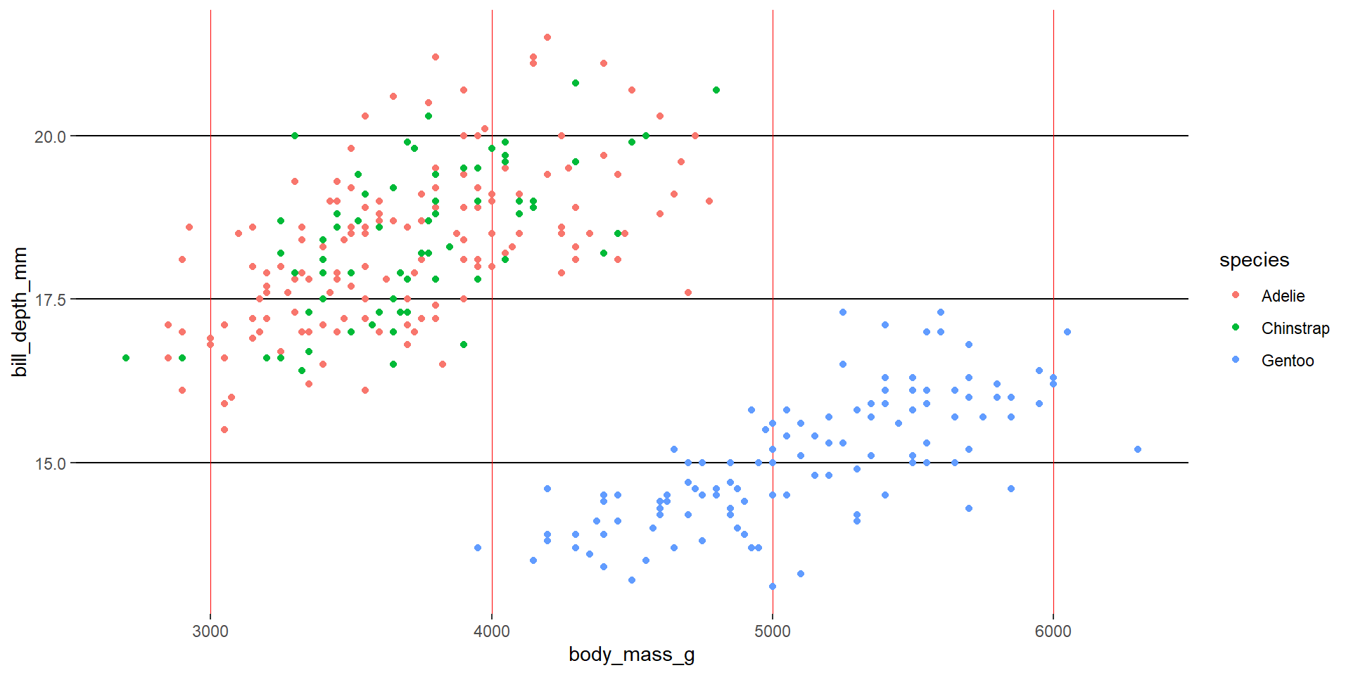
Hierarchichal modifications
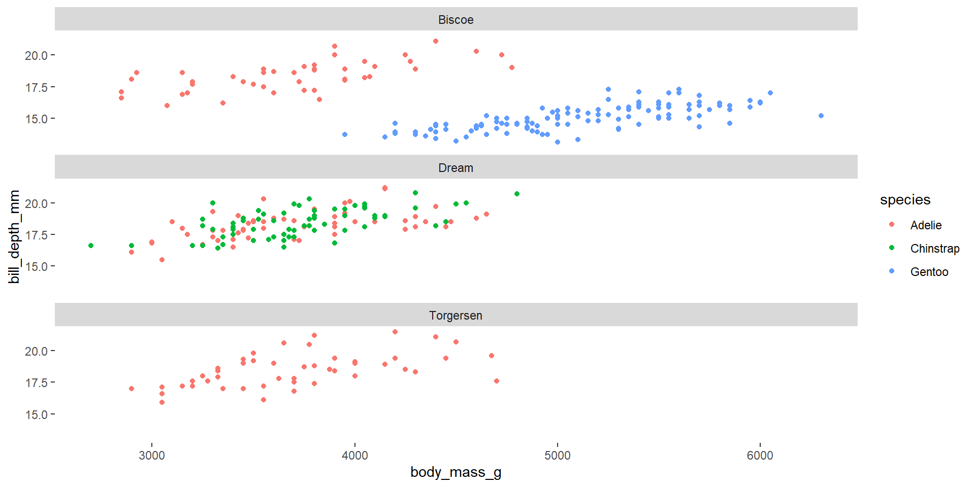
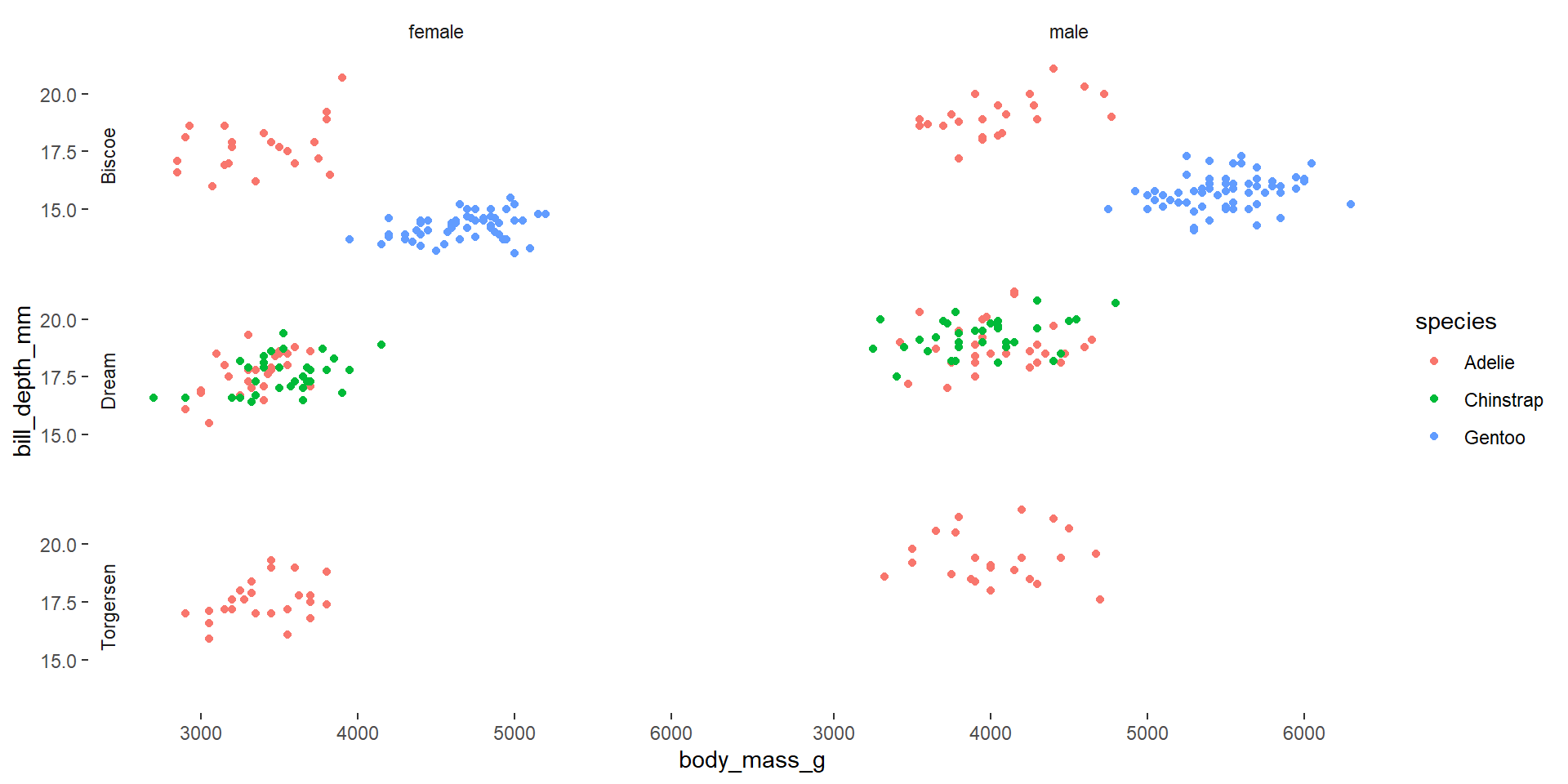
facet_wrap
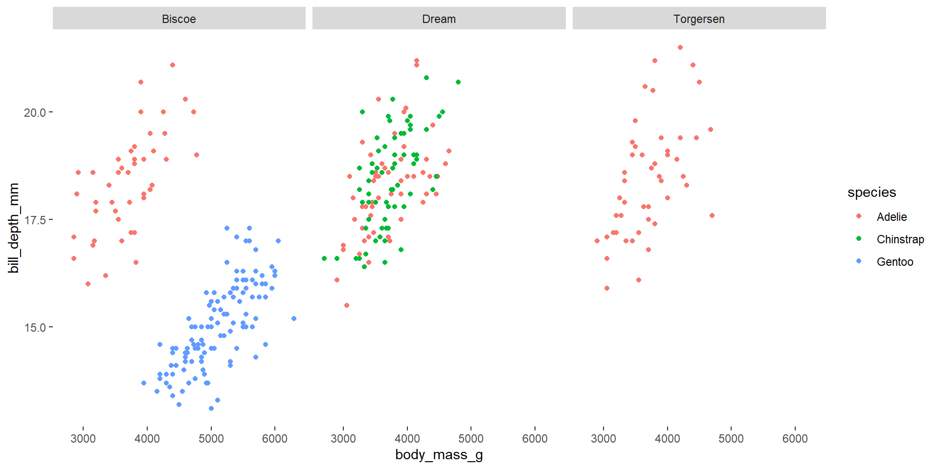
facet_wrap
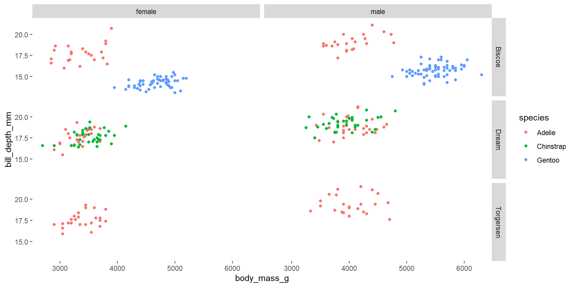
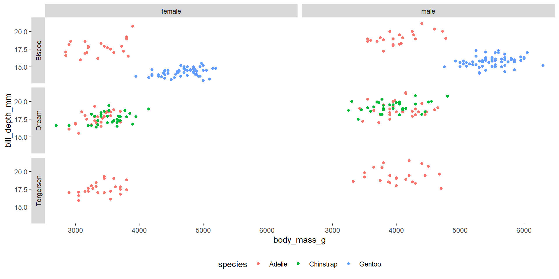
facet_grid
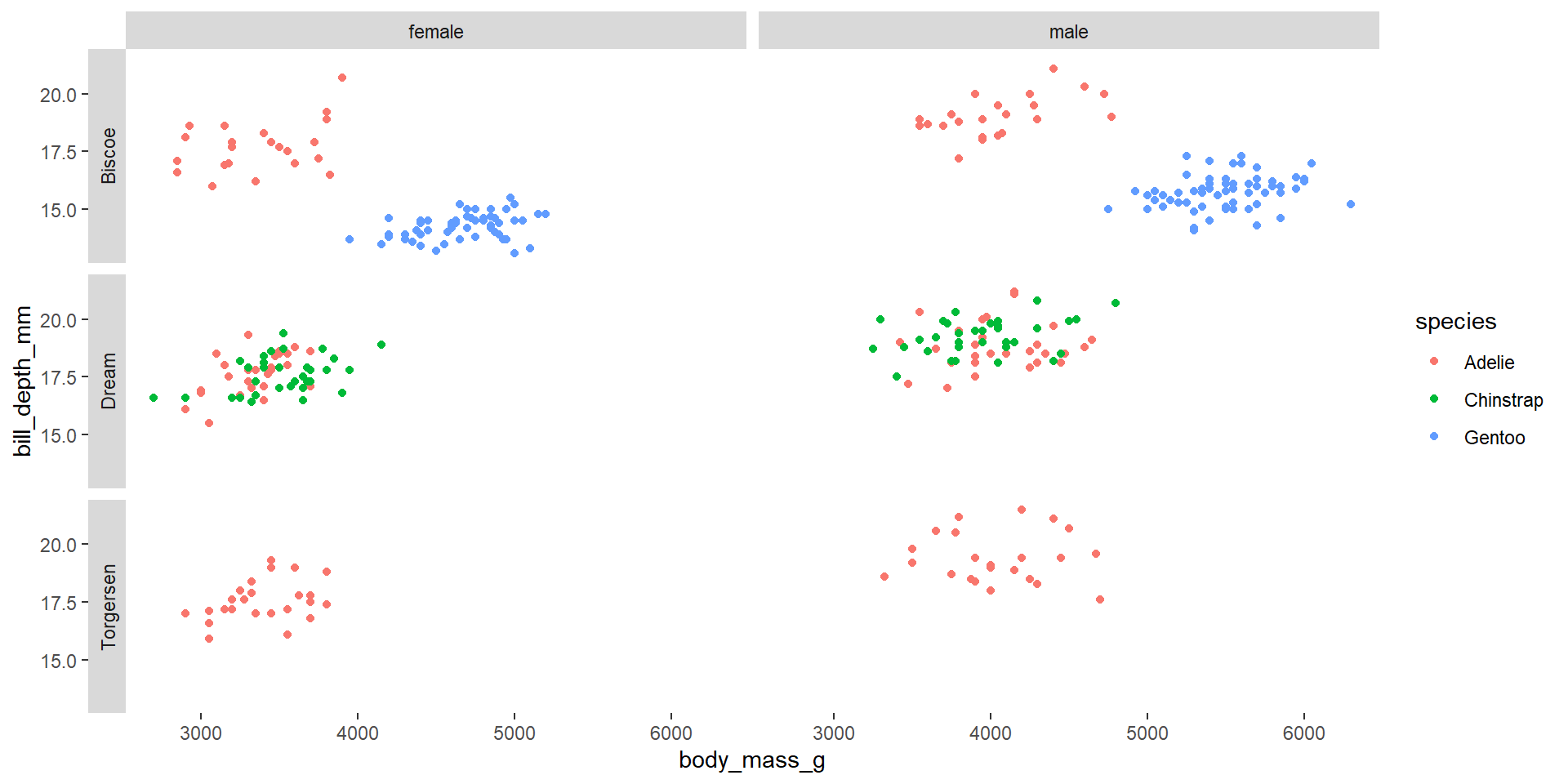
Modify facet label placement
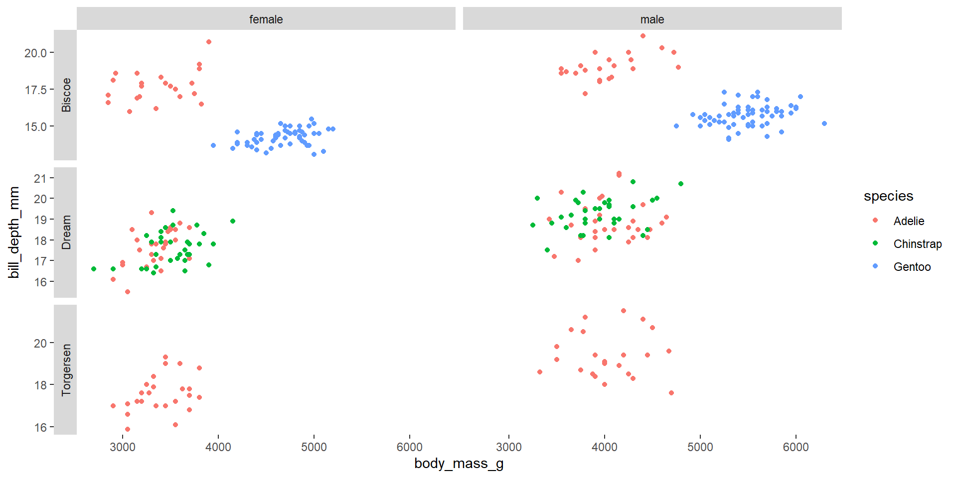
Modify facet scales
Modify facet strip options
Move the legend
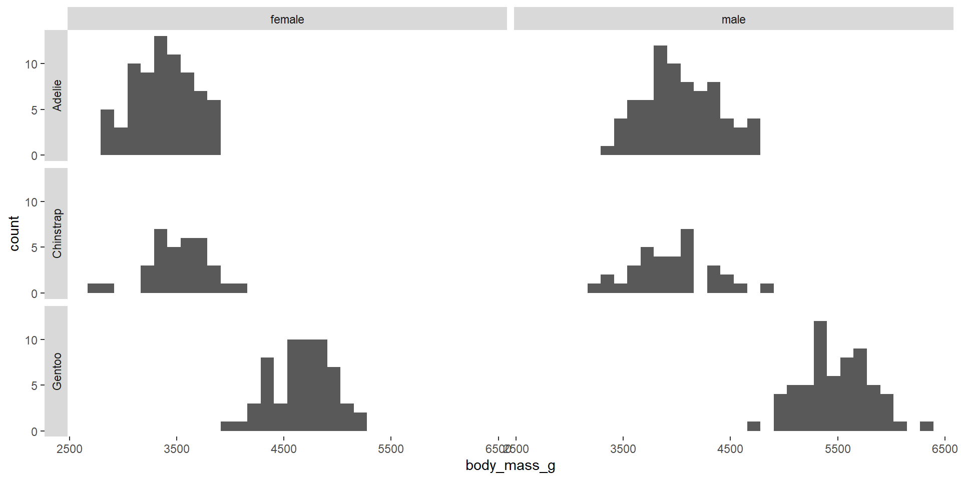
Counterintuitive marks and channels
Size is much worse than position for showing continuous data!
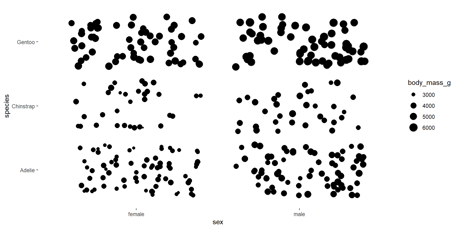
Counterintuitive marks and channels
Size is much worse than position for showing continuous data!
Marks and channels: Options
Shape is less effective than color for differentiating categories!
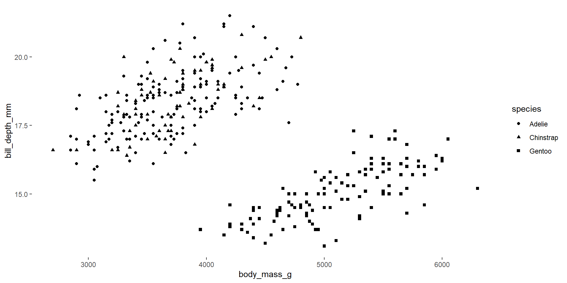
Marks and channels: Options
Shape is less effective than color for differentiating categories!

cols4all