Categorical models and model comparison

Adding categorical predictors

library(palmerpenguins)
library(dplyr)

Attaching package: 'dplyr'

The following objects are masked from 'package:stats':

    filter, lag

The following objects are masked from 'package:base':

    intersect, setdiff, setequal, union

library(ggplot2)
library(ggdist)
library(brms)

Loading required package: Rcpp

Loading 'brms' package (version 2.21.0). Useful instructions
can be found by typing help('brms'). A more detailed introduction
to the package is available through vignette('brms_overview').

Attaching package: 'brms'

The following objects are masked from 'package:ggdist':

    dstudent_t, pstudent_t, qstudent_t, rstudent_t

The following object is masked from 'package:stats':

    ar

library(tidybayes)

Attaching package: 'tidybayes'

The following objects are masked from 'package:brms':

    dstudent_t, pstudent_t, qstudent_t, rstudent_t

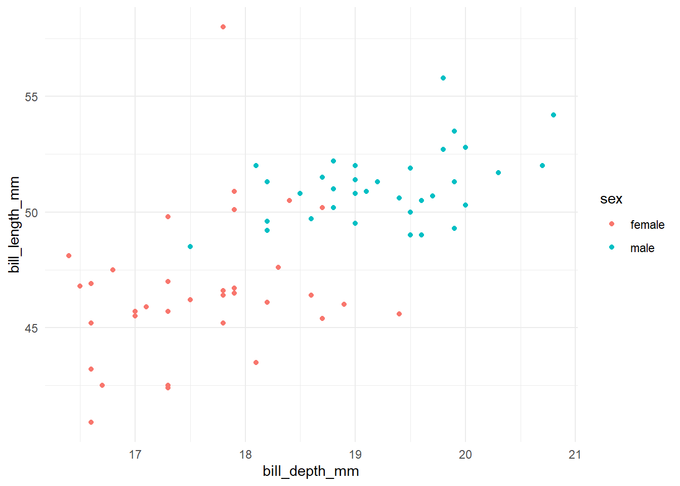
library(tidyr)
theme_set(theme_minimal())

penguins <- penguins |>
  filter(!is.na(sex),
         species == "Chinstrap") 

ggplot(penguins, aes(bill_depth_mm, 
                     bill_length_mm, 
                     color = sex)) +
  geom_point()

The model

• Say we want to model bill_length as a function of both bill_depth and sex.
• There are different approaches to adding a categorial predictor to a model, sometimes called “indicator” (or “dummy”) variables, or “index” variables. McElreath comes down strongly in favor of using “index” variables. For more discussion, see here and links therein.

The code

Fitting the model

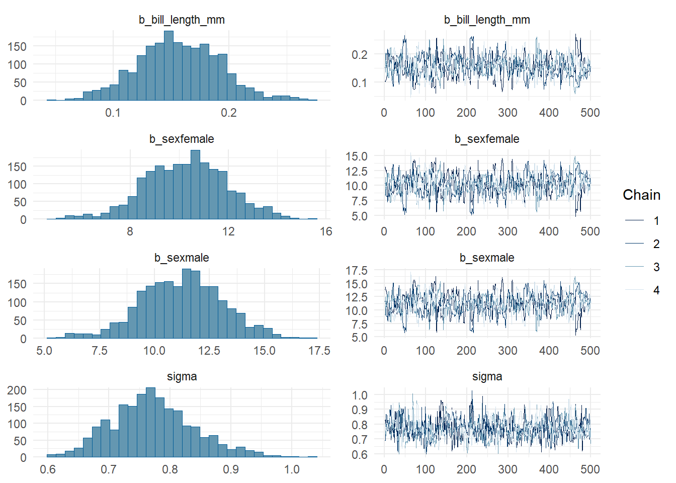
First we can fit a model that will just fit different intercepts for the different species:

depth_length_sex_brm <- brm(
  family = gaussian,
  data = penguins,
  formula = bill_depth_mm ~ 0 + bill_length_mm + sex,
  prior = c(
      prior(normal(0, 5), class = b),
      prior(uniform(0, 20), class = sigma, ub = 20)),
  iter = 1000
)

Interpreting the model

Model diagnostics:

summary(depth_length_sex_brm)

 Family: gaussian 
  Links: mu = identity; sigma = identity 
Formula: bill_depth_mm ~ 0 + bill_length_mm + sex 
   Data: penguins (Number of observations: 68) 
  Draws: 4 chains, each with iter = 1000; warmup = 500; thin = 1;
         total post-warmup draws = 2000

Regression Coefficients:
               Estimate Est.Error l-95% CI u-95% CI Rhat Bulk_ESS Tail_ESS
bill_length_mm     0.16      0.04     0.09     0.23 1.01      356      391
sexfemale         10.28      1.67     7.00    13.64 1.01      356      399
sexmale           11.24      1.83     7.60    14.84 1.01      361      388

Further Distributional Parameters:
      Estimate Est.Error l-95% CI u-95% CI Rhat Bulk_ESS Tail_ESS
sigma     0.77      0.07     0.65     0.92 1.00      545      664

Draws were sampled using sampling(NUTS). For each parameter, Bulk_ESS
and Tail_ESS are effective sample size measures, and Rhat is the potential
scale reduction factor on split chains (at convergence, Rhat = 1).

plot(depth_length_sex_brm)

Comparing the intercepts for sex:

as_draws_df(depth_length_sex_brm) %>% 
  mutate(diff_fm = b_sexfemale - b_sexmale) %>% 
  pivot_longer(cols = c(b_sexfemale:sigma, diff_fm)) %>% 
  group_by(name) %>% 
  mean_qi(value, .width = .89)

Warning: Dropping 'draws_df' class as required metadata was removed.

# A tibble: 4 × 7
  name         value .lower .upper .width .point .interval
  <chr>        <dbl>  <dbl>  <dbl>  <dbl> <chr>  <chr>    
1 b_sexfemale 10.3    7.64  12.9     0.89 mean   qi       
2 b_sexmale   11.2    8.31  14.1     0.89 mean   qi       
3 diff_fm     -0.960 -1.34  -0.564   0.89 mean   qi       
4 sigma        0.772  0.670  0.889   0.89 mean   qi       

Model comparison

See chapter 7 and the bookdown book here for more on model comparison criteria.

depth_length_sex_brm <- depth_length_sex_brm |> add_criterion(criterion = c("waic", "loo"))

Warning: 
2 (2.9%) p_waic estimates greater than 0.4. We recommend trying loo instead.

depth_length_sex_brm$criteria

$waic

Computed from 2000 by 68 log-likelihood matrix.

          Estimate   SE
elpd_waic    -80.2  5.7
p_waic         4.1  1.3
waic         160.3 11.3

2 (2.9%) p_waic estimates greater than 0.4. We recommend trying loo instead. 

$loo

Computed from 2000 by 68 log-likelihood matrix.

         Estimate   SE
elpd_loo    -80.3  5.7
p_loo         4.2  1.4
looic       160.5 11.4
------
MCSE of elpd_loo is 0.2.
MCSE and ESS estimates assume MCMC draws (r_eff in [0.2, 1.1]).

All Pareto k estimates are good (k < 0.7).
See help('pareto-k-diagnostic') for details.

Compare this to our old model, with no term for sex:

depth_length_brm <- depth_length_brm |> add_criterion(criterion = c("waic", "loo"))

Warning: 
1 (1.5%) p_waic estimates greater than 0.4. We recommend trying loo instead.

depth_length_brm$criteria

$waic

Computed from 2000 by 68 log-likelihood matrix.

          Estimate   SE
elpd_waic    -89.2  6.8
p_waic         3.6  1.7
waic         178.4 13.5

1 (1.5%) p_waic estimates greater than 0.4. We recommend trying loo instead. 

$loo

Computed from 2000 by 68 log-likelihood matrix.

         Estimate   SE
elpd_loo    -89.2  6.8
p_loo         3.6  1.7
looic       178.4 13.5
------
MCSE of elpd_loo is 0.1.
MCSE and ESS estimates assume MCMC draws (r_eff in [0.7, 1.0]).

All Pareto k estimates are good (k < 0.7).
See help('pareto-k-diagnostic') for details.