Fitting and interpreting interaction models

New dataset: this time with mice!

The Portal data

The Portal Project: 40 years of population surveys of rodents in southeastern Arizona.

We’ll focus on abundance trends in two species, Dipodomys spectabilis and Chaetodipus penicillatus. More on these species.

Getting the Portal teaching data

install.packages('ratdat')

Plotting trends in DS and PP

library(ratdat)

Warning: package 'ratdat' was built under R version 4.4.1

library(dplyr)

Attaching package: 'dplyr'

The following objects are masked from 'package:stats':

    filter, lag

The following objects are masked from 'package:base':

    intersect, setdiff, setequal, union

library(ggplot2)
library(ggdist)
library(brms)

Loading required package: Rcpp

Loading 'brms' package (version 2.21.0). Useful instructions
can be found by typing help('brms'). A more detailed introduction
to the package is available through vignette('brms_overview').

Attaching package: 'brms'

The following objects are masked from 'package:ggdist':

    dstudent_t, pstudent_t, qstudent_t, rstudent_t

The following object is masked from 'package:stats':

    ar

library(tidybayes)

Attaching package: 'tidybayes'

The following objects are masked from 'package:brms':

    dstudent_t, pstudent_t, qstudent_t, rstudent_t

library(tidyr)
theme_set(theme_minimal())

complete_annual <- ratdat::complete |>
  group_by(year, species_id) |>
  filter(species_id %in% c("DS", "PP")) |>
  tally() |>
  ungroup() |>
  mutate(n = scale(n))

ggplot(complete_annual, aes(year, n, color = species_id)) +
  geom_point()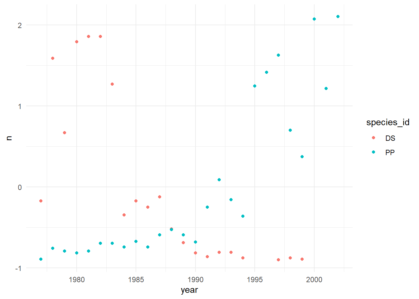

Fitting models

• Say we want to model abund as a function of time, and we are curious how species affects this relationship

abund and species (but no interaction)

abund_species_brm <- brm(
  family = gaussian,
  data = complete_annual,
  formula = n ~ 0 + year + species_id,
  iter = 4000, 
  warmup = 1000, 
  chains = 4, 
  cores = 4,
  seed = 1977,
  file = "abund_species_brm",
  control = list(max_treedepth = 15)
)

abund and species with interaction

abund_species_interaction_brm <-  brm(data = complete_annual, 
      family = gaussian,
      bf(n ~ 0 + a + b * year, 
         a ~ 0 + species_id,
         b ~ 0 + species_id,
         nl = TRUE),
      iter = 4000, 
      warmup = 1000, 
      chains = 4, 
      cores = 4,
      control = list(max_treedepth = 15),
      seed = 8,
      file = "abund_species_interaction_brm")

A note on priors

default_prior(abund_species_brm)

                prior class         coef group resp dpar nlpar lb ub
               (flat)     b                                         
               (flat)     b species_idDS                            
               (flat)     b species_idPP                            
               (flat)     b         year                            
 student_t(3, 0, 2.5) sigma                                     0   
       source
      default
 (vectorized)
 (vectorized)
 (vectorized)
      default

default_prior(abund_species_interaction_brm)

                prior class         coef group resp dpar nlpar lb ub
               (flat)     b                                  a      
               (flat)     b species_idDS                     a      
               (flat)     b species_idPP                     a      
               (flat)     b                                  b      
               (flat)     b species_idDS                     b      
               (flat)     b species_idPP                     b      
 student_t(3, 0, 2.5) sigma                                     0   
       source
      default
 (vectorized)
 (vectorized)
      default
 (vectorized)
 (vectorized)
      default

Model results

No interaction

summary(abund_species_brm)

 Family: gaussian 
  Links: mu = identity; sigma = identity 
Formula: n ~ 0 + year + species_id 
   Data: complete_annual (Number of observations: 47) 
  Draws: 4 chains, each with iter = 4000; warmup = 1000; thin = 1;
         total post-warmup draws = 12000

Regression Coefficients:
             Estimate Est.Error l-95% CI u-95% CI Rhat Bulk_ESS Tail_ESS
year             0.02      0.02    -0.02     0.07 1.00     1918     2020
species_idDS   -46.08     42.89  -131.69    36.68 1.00     1919     2016
species_idPP   -46.12     42.94  -131.86    36.60 1.00     1918     2019

Further Distributional Parameters:
      Estimate Est.Error l-95% CI u-95% CI Rhat Bulk_ESS Tail_ESS
sigma     1.03      0.12     0.83     1.29 1.00     2919     2884

Draws were sampled using sampling(NUTS). For each parameter, Bulk_ESS
and Tail_ESS are effective sample size measures, and Rhat is the potential
scale reduction factor on split chains (at convergence, Rhat = 1).

plot(abund_species_brm)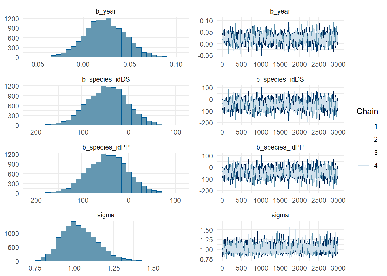

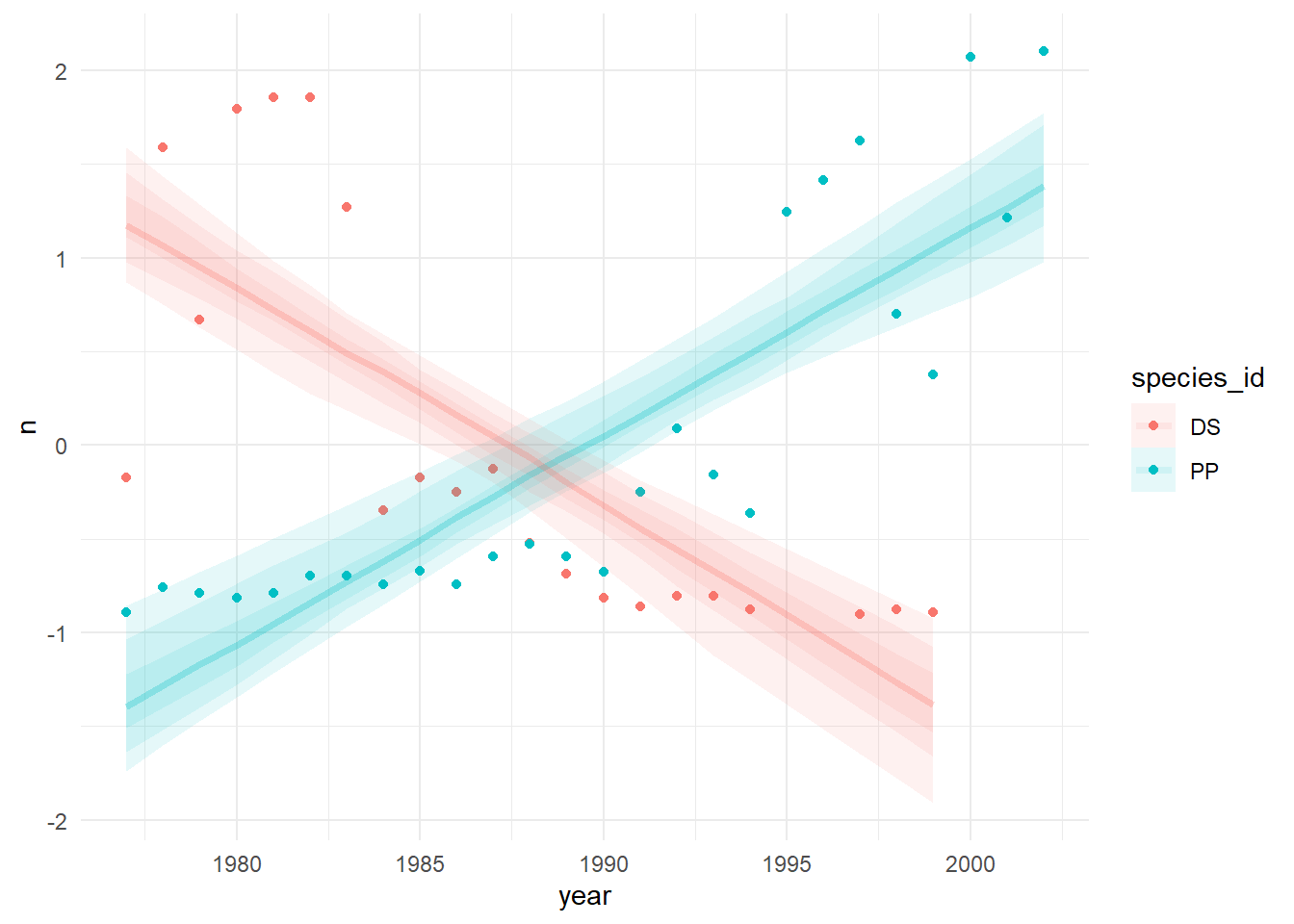
abund_species_brm_predictions <- complete_annual |>
  add_epred_draws(abund_species_brm, ndraws = 50)

ggplot(abund_species_brm_predictions, aes(year, n, color = species_id, fill = species_id)) +
  geom_point() +  
  stat_lineribbon(aes(y = .epred), alpha = .1)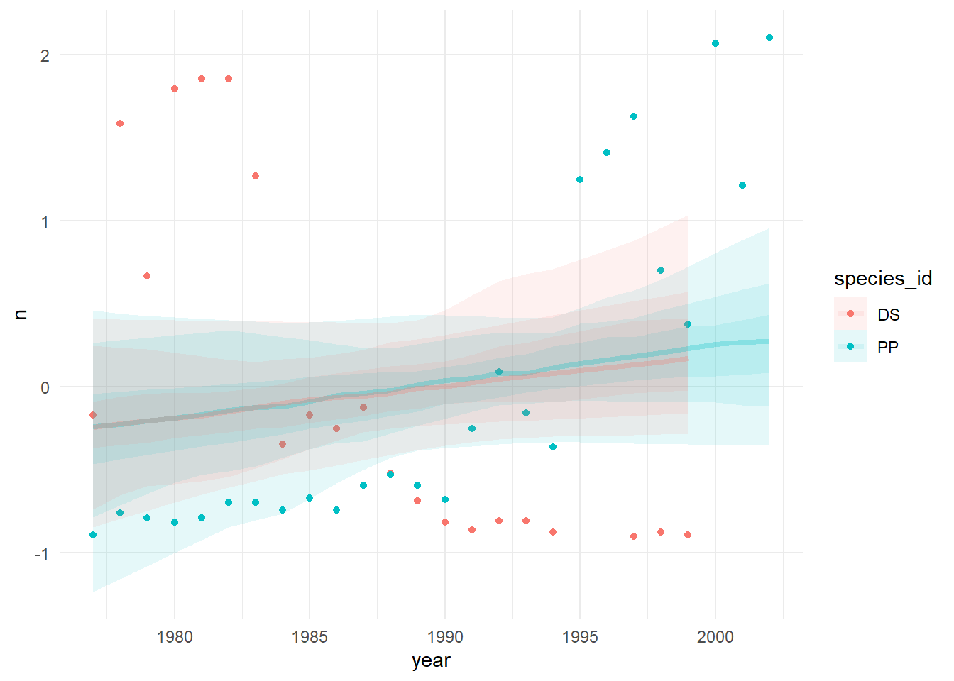 

Interaction

summary(abund_species_interaction_brm)

 Family: gaussian 
  Links: mu = identity; sigma = identity 
Formula: n ~ 0 + a + b * year 
         a ~ 0 + species_id
         b ~ 0 + species_id
   Data: complete_annual (Number of observations: 47) 
  Draws: 4 chains, each with iter = 4000; warmup = 1000; thin = 1;
         total post-warmup draws = 12000

Regression Coefficients:
               Estimate Est.Error l-95% CI u-95% CI Rhat Bulk_ESS Tail_ESS
a_species_idDS   237.47     40.99   157.80   318.19 1.00     4569     4924
a_species_idPP  -220.30     31.96  -284.72  -154.73 1.00     4501     4600
b_species_idDS    -0.12      0.02    -0.16    -0.08 1.00     4570     4953
b_species_idPP     0.11      0.02     0.08     0.14 1.00     4499     4544

Further Distributional Parameters:
      Estimate Est.Error l-95% CI u-95% CI Rhat Bulk_ESS Tail_ESS
sigma     0.62      0.07     0.50     0.77 1.00     5474     4694

Draws were sampled using sampling(NUTS). For each parameter, Bulk_ESS
and Tail_ESS are effective sample size measures, and Rhat is the potential
scale reduction factor on split chains (at convergence, Rhat = 1).

plot(abund_species_interaction_brm)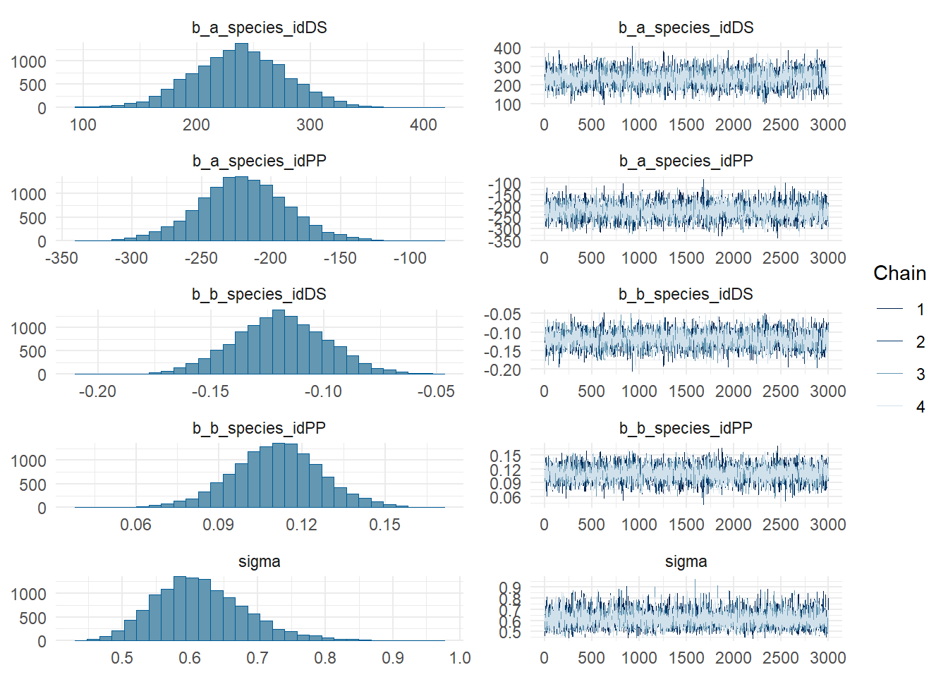

abund_species_interaction_brm_draws <- tidy_draws(abund_species_interaction_brm)

ggplot(abund_species_interaction_brm_draws, aes(b_b_species_idDS - b_b_species_idPP)) +
  geom_histogram()

`stat_bin()` using `bins = 30`. Pick better value with `binwidth`.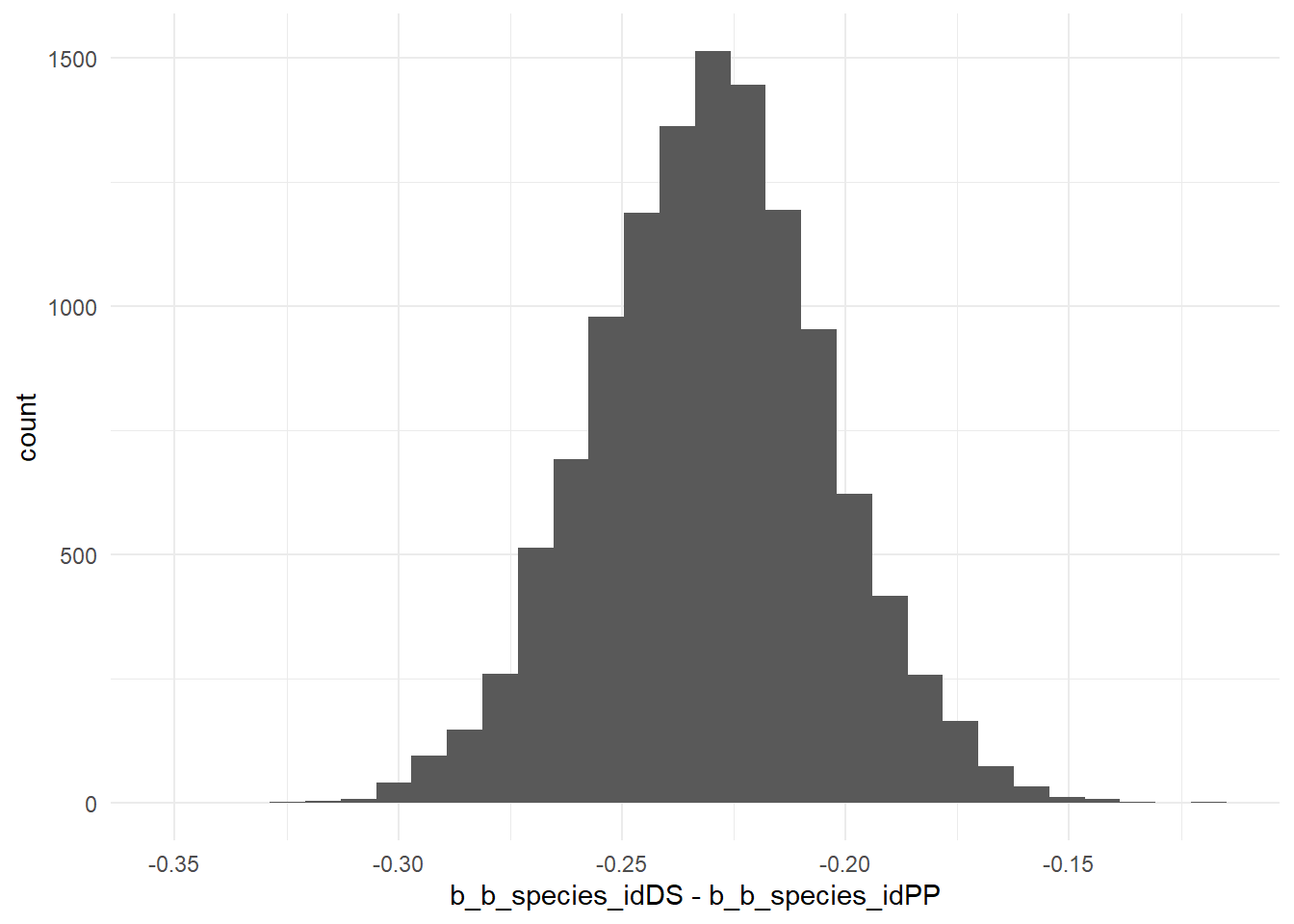

abund_species_interaction_brm_predictions <- complete_annual |>
  add_epred_draws(abund_species_interaction_brm, ndraws = 50)

ggplot(abund_species_interaction_brm_predictions, aes(year, n, color = species_id, fill = species_id)) +
  geom_point() +  
  stat_lineribbon(aes(y = .epred), alpha = .1)