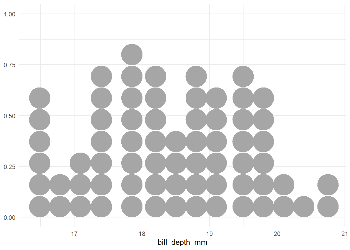
This just says that bill depth is normally distributed with some mean and some standard deviation. We can observe bill depth (data), but we don’t know the mean or standard deviation (parameters).
For the parameters, we need priors.
\(\mu \sim N(50, 15)\)
This is to say that \(\mu\) is some number drawn from a normal distribution centered on 50:
data.frame(mu =rnorm(1000, mean =20, sd =6)) |>ggplot(aes(x = mu)) +geom_dotsinterval() +ggtitle("Simulations from prior for mu")
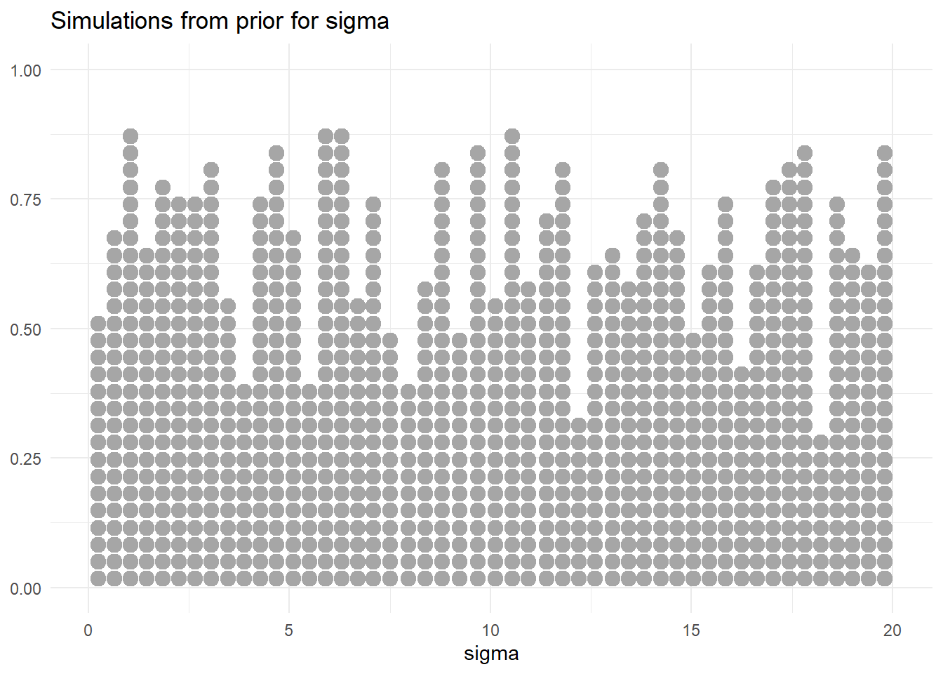
$(0, 20)$
And here we’re saying that we figure \(sigma\) is potentially uniformly distributed ranging from 0-20. Standard deviations have to be positive, and otherwise this is a very broad range.
data.frame(sigma =runif(1000, 0, 20)) |>ggplot(aes(x = sigma)) +geom_dotsinterval() +ggtitle("Simulations from prior for sigma")
Exploring the generative model
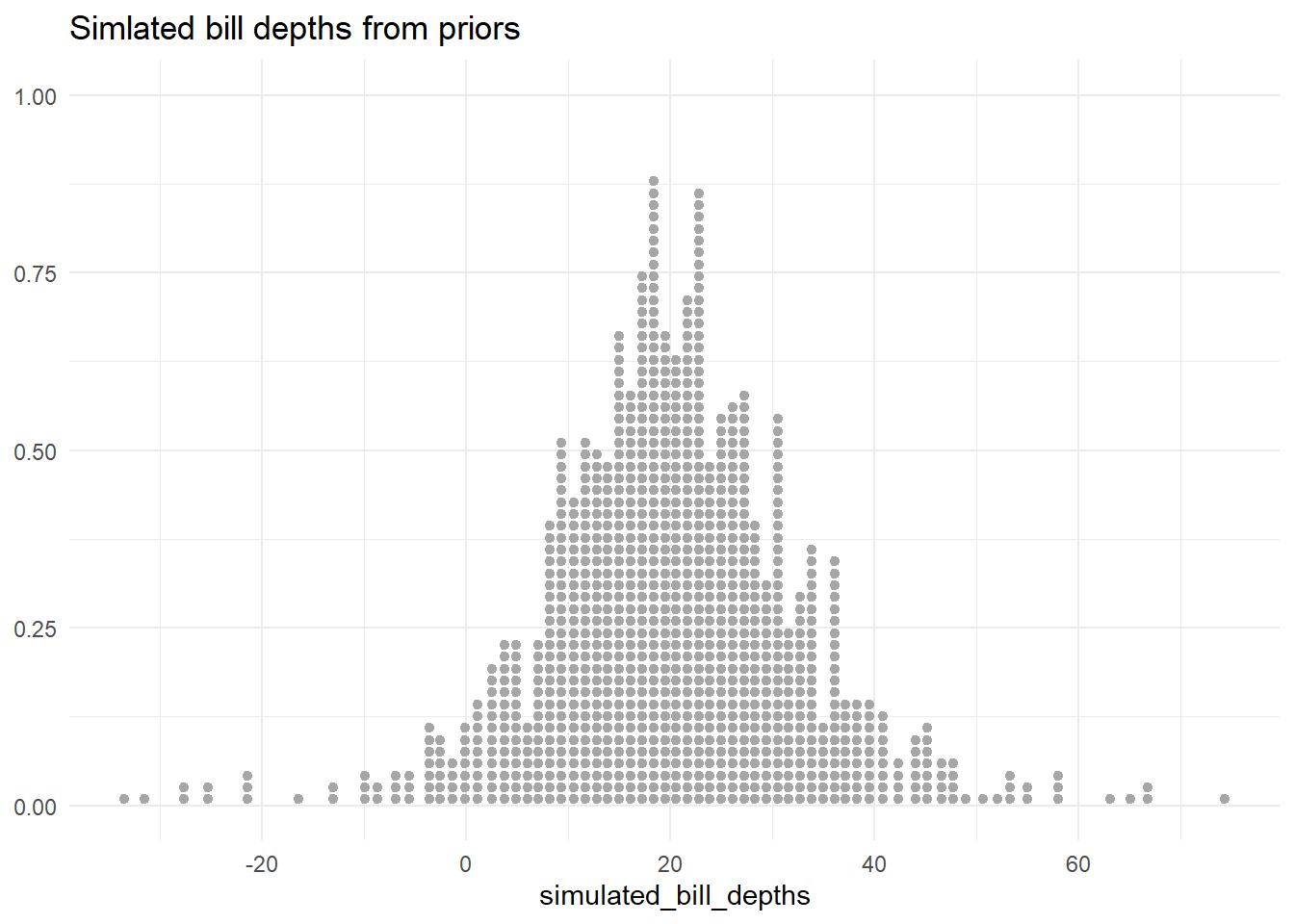
sample_mu <-rnorm(1000, 20, 6)sample_sigmas <-runif(1000, 0, 20)data.frame(simulated_bill_depths =rnorm(1000, sample_mu, sample_sigmas)) |>ggplot(aes(simulated_bill_depths)) +geom_dotsinterval() +ggtitle("Simlated bill depths from priors")
This is our simulation of expected bill depths before explicitly taking into account the data (although we did look at the density plot before specifying the priors).
Taking into account the data
See here for translations of rethinking code to brms.
Loading 'brms' package (version 2.21.0). Useful instructions
can be found by typing help('brms'). A more detailed introduction
to the package is available through vignette('brms_overview').
Attaching package: 'brms'
The following objects are masked from 'package:ggdist':

    dstudent_t, pstudent_t, qstudent_t, rstudent_t
The following object is masked from 'package:stats':

    ar
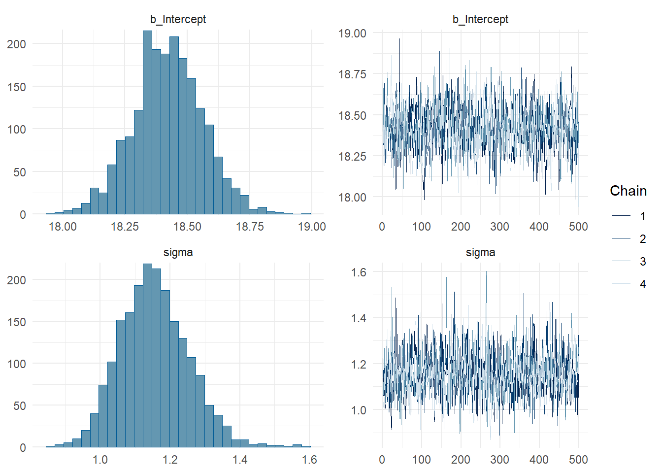
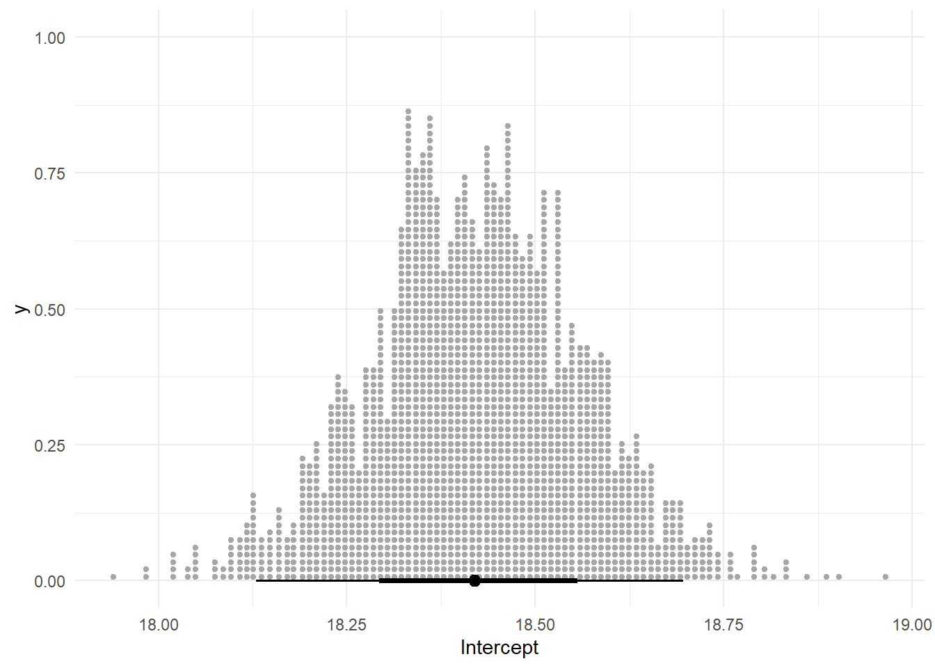
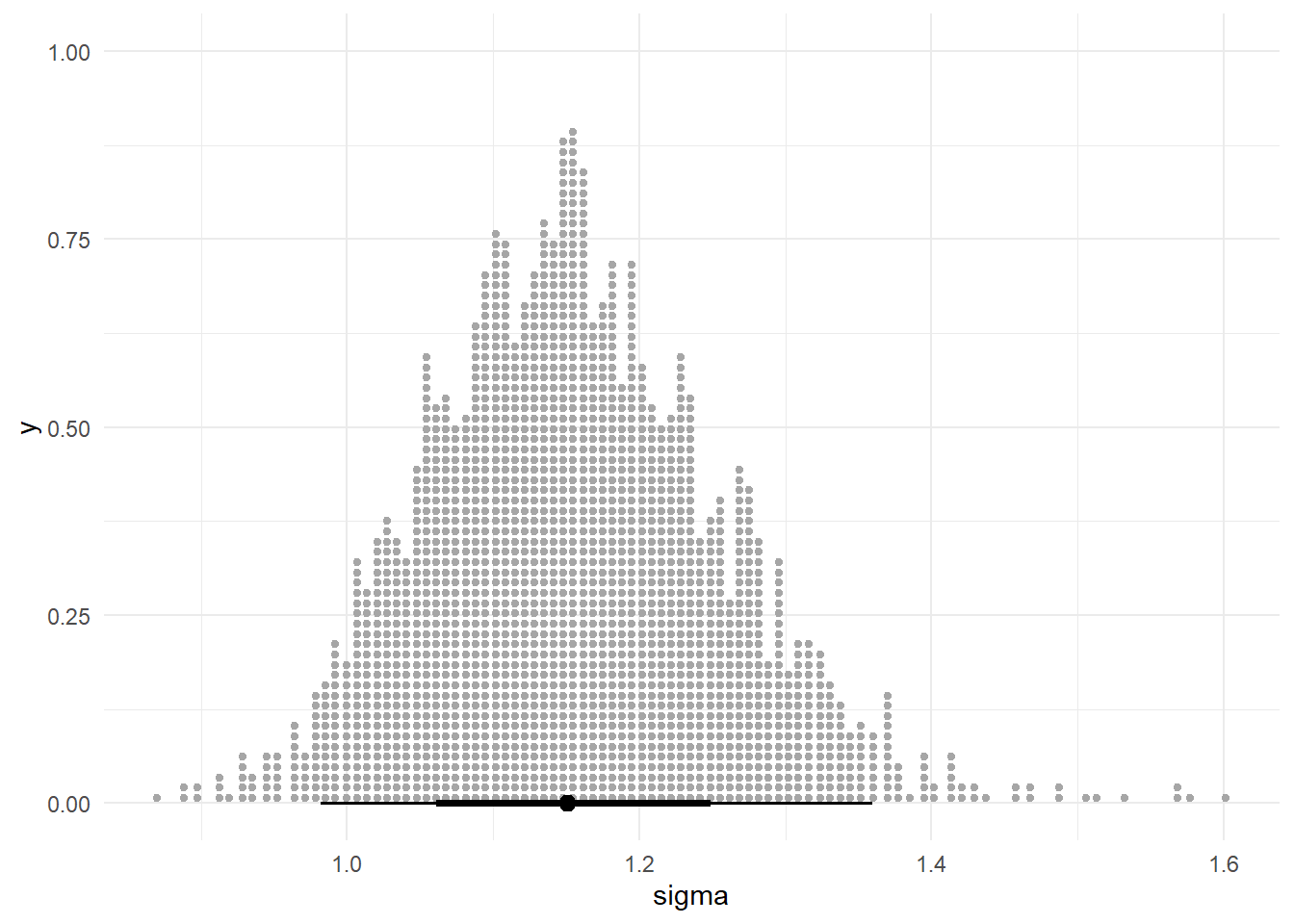
plot(bill_depth_brm)
summary(bill_depth_brm)
 Family: gaussian
  Links: mu = identity; sigma = identity
Formula: bill_depth_mm ~ 1
   Data: penguins (Number of observations: 68)
  Draws: 4 chains, each with iter = 1000; warmup = 500; thin = 1;
         total post-warmup draws = 2000

Regression Coefficients:
          Estimate Est.Error l-95% CI u-95% CI Rhat Bulk_ESS Tail_ESS
Intercept    18.42      0.14    18.13    18.70 1.00     1390     1244

Further Distributional Parameters:
      Estimate Est.Error l-95% CI u-95% CI Rhat Bulk_ESS Tail_ESS
sigma     1.16      0.10     0.98     1.36 1.00     1501     1307

Draws were sampled using sampling(NUTS). For each parameter, Bulk_ESS
and Tail_ESS are effective sample size measures, and Rhat is the potential
scale reduction factor on split chains (at convergence, Rhat = 1).
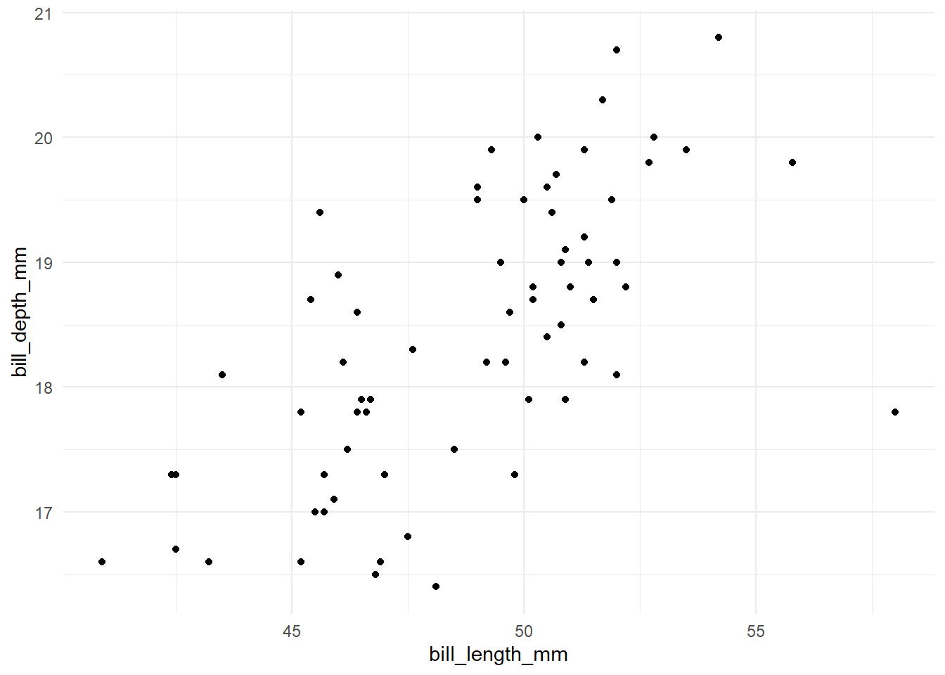
This addition makes it into a linear model. Instead of estimating \(\mu\) from the data, we say that the mean of bill depth varies with bill length as linear function with an intercept \(\alpha\) and a slope \(\beta\).
\(\alpha\) and \(\beta\) are now additional parameters that we will estimate and therefore need to set priors for.
ggplot(prior_draw, aes(bill_length, mu)) +geom_line() +geom_ribbon(aes(ymin = mu - sigma,ymax = mu + sigma),alpha = .3) +geom_point(aes(y = sim_depth)) +ggtitle("Simulated bill depths",subtitle ="Based on a single draw from the priors")
Fitting the model (with data)
depth_length_brm <-brm(family = gaussian,data = penguins,formula = bill_depth_mm ~ bill_length_mm,prior =c(prior(normal(20, 6), class = Intercept),prior(normal(0, 5), class = b),prior(uniform(0, 20), class = sigma, ub =20)),iter =1000)
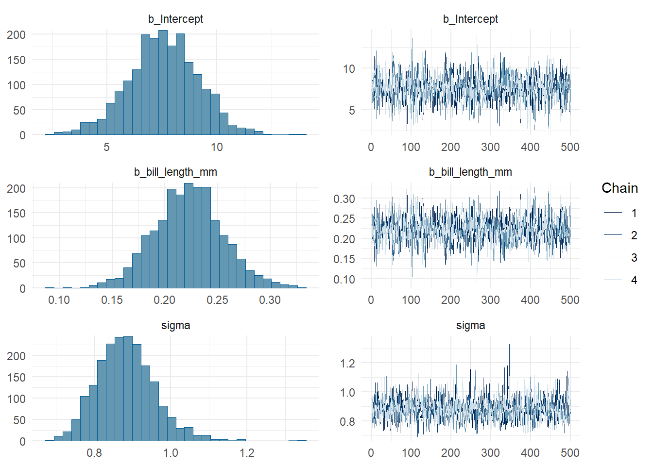
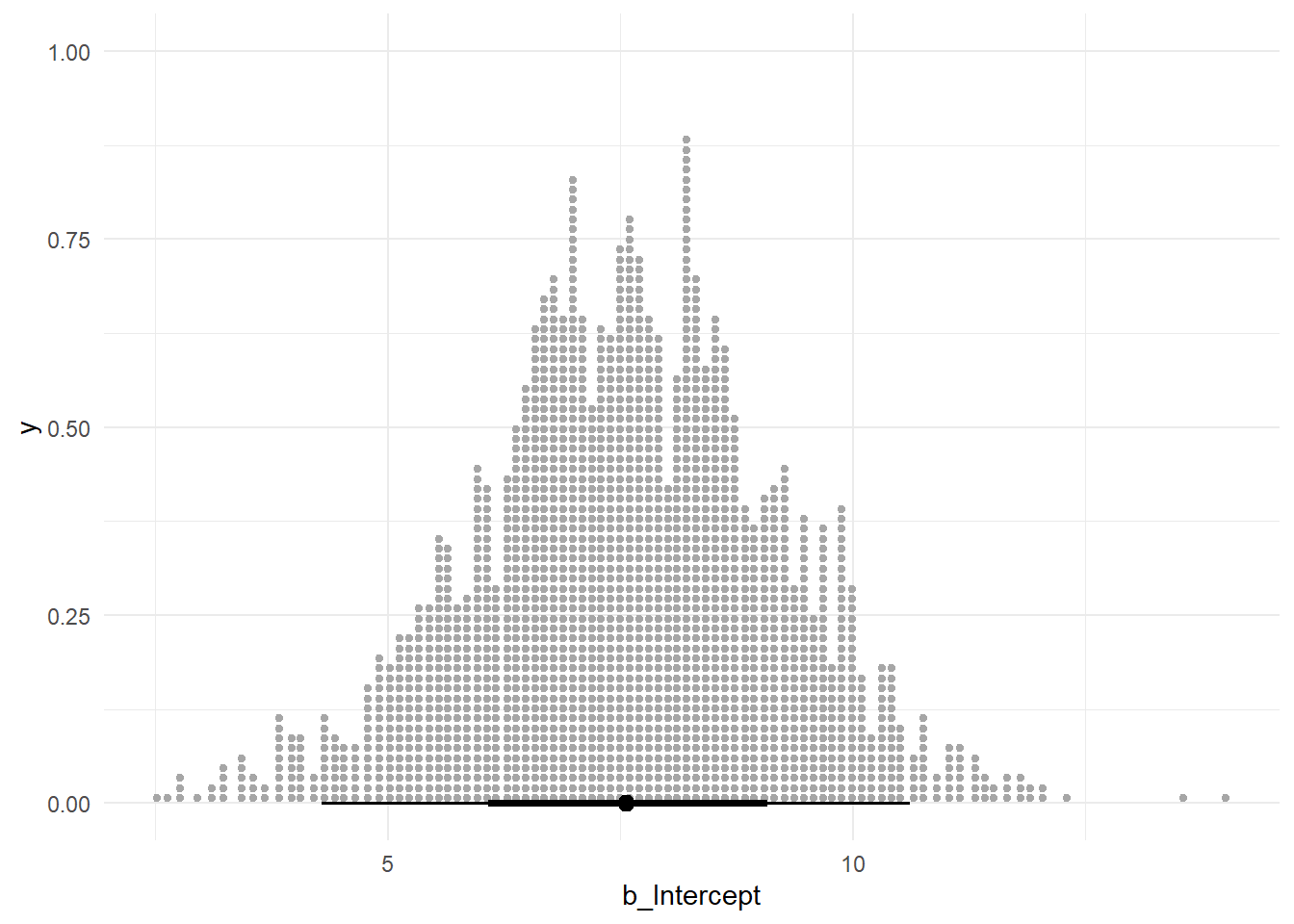
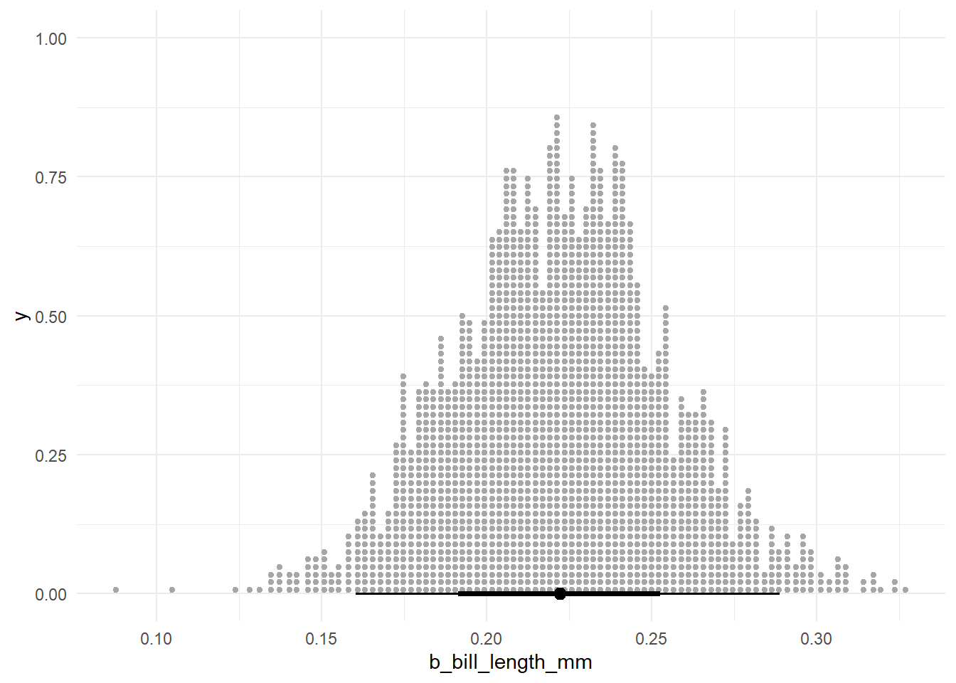
plot(depth_length_brm)
summary(depth_length_brm)
 Family: gaussian
  Links: mu = identity; sigma = identity
Formula: bill_depth_mm ~ bill_length_mm
   Data: penguins (Number of observations: 68)
  Draws: 4 chains, each with iter = 1000; warmup = 500; thin = 1;
         total post-warmup draws = 2000

Regression Coefficients:
               Estimate Est.Error l-95% CI u-95% CI Rhat Bulk_ESS Tail_ESS
Intercept          7.57      1.60     4.29    10.62 1.00     1828     1302
bill_length_mm     0.22      0.03     0.16     0.29 1.00     1803     1301

Further Distributional Parameters:
      Estimate Est.Error l-95% CI u-95% CI Rhat Bulk_ESS Tail_ESS
sigma     0.88      0.08     0.75     1.05 1.00     2180     1472

Draws were sampled using sampling(NUTS). For each parameter, Bulk_ESS
and Tail_ESS are effective sample size measures, and Rhat is the potential
scale reduction factor on split chains (at convergence, Rhat = 1).