Posterior distributions

Getting a toy model

See the model from last week:

library(palmerpenguins)
library(dplyr)


Attaching package: 'dplyr'

The following objects are masked from 'package:stats':

    filter, lag

The following objects are masked from 'package:base':

    intersect, setdiff, setequal, union

library(ggplot2)
library(ggdist)
theme_set(theme_minimal())

penguins <- penguins |>
  filter(!is.na(sex)) |>
  filter(species == "Chinstrap") 

ggplot(penguins, aes(bill_length_mm, 
                     bill_depth_mm)) +
  geom_point()

The model

\(\text{billdepth}_i \sim N(\mu, \sigma)\)

\(\mu_i = \alpha + \beta(\text{billlength}_i - \text{mean}(\text{billlength}))\)

\(\alpha \sim N(20, 6)\)

\(\beta \sim N(0, 5)\)

\(\sigma \sim \text{Uniform}(0, 20)\)

The code

Fitting the model (with data)

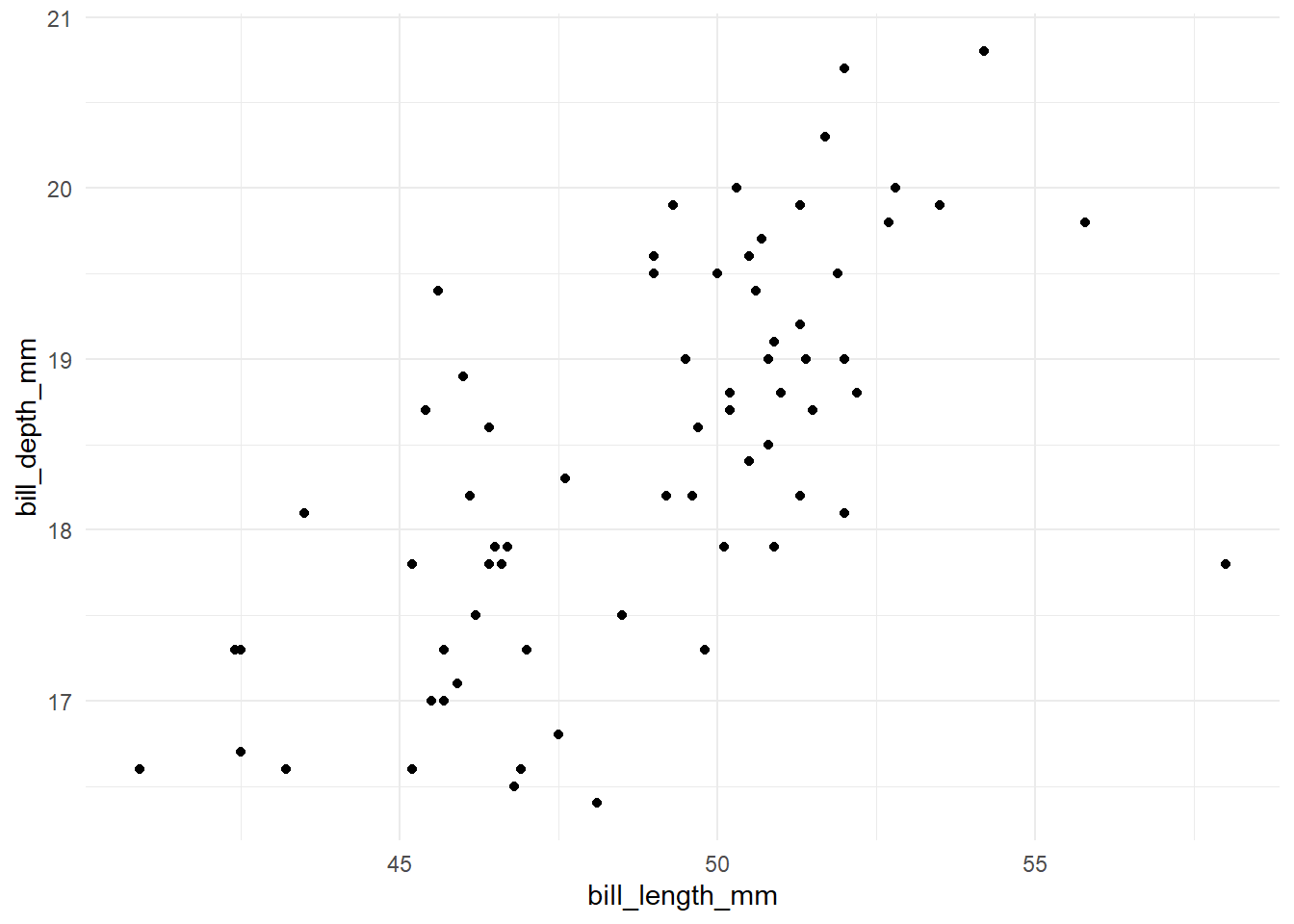
depth_length_brm <- brm(
  family = gaussian,
  data = penguins,
  formula = bill_depth_mm ~ bill_length_mm,
  prior = c(
      prior(normal(20, 6), class = Intercept),
      prior(normal(0, 5), class = b),
      prior(uniform(0, 20), class = sigma, ub = 20)),
  iter = 1000
)

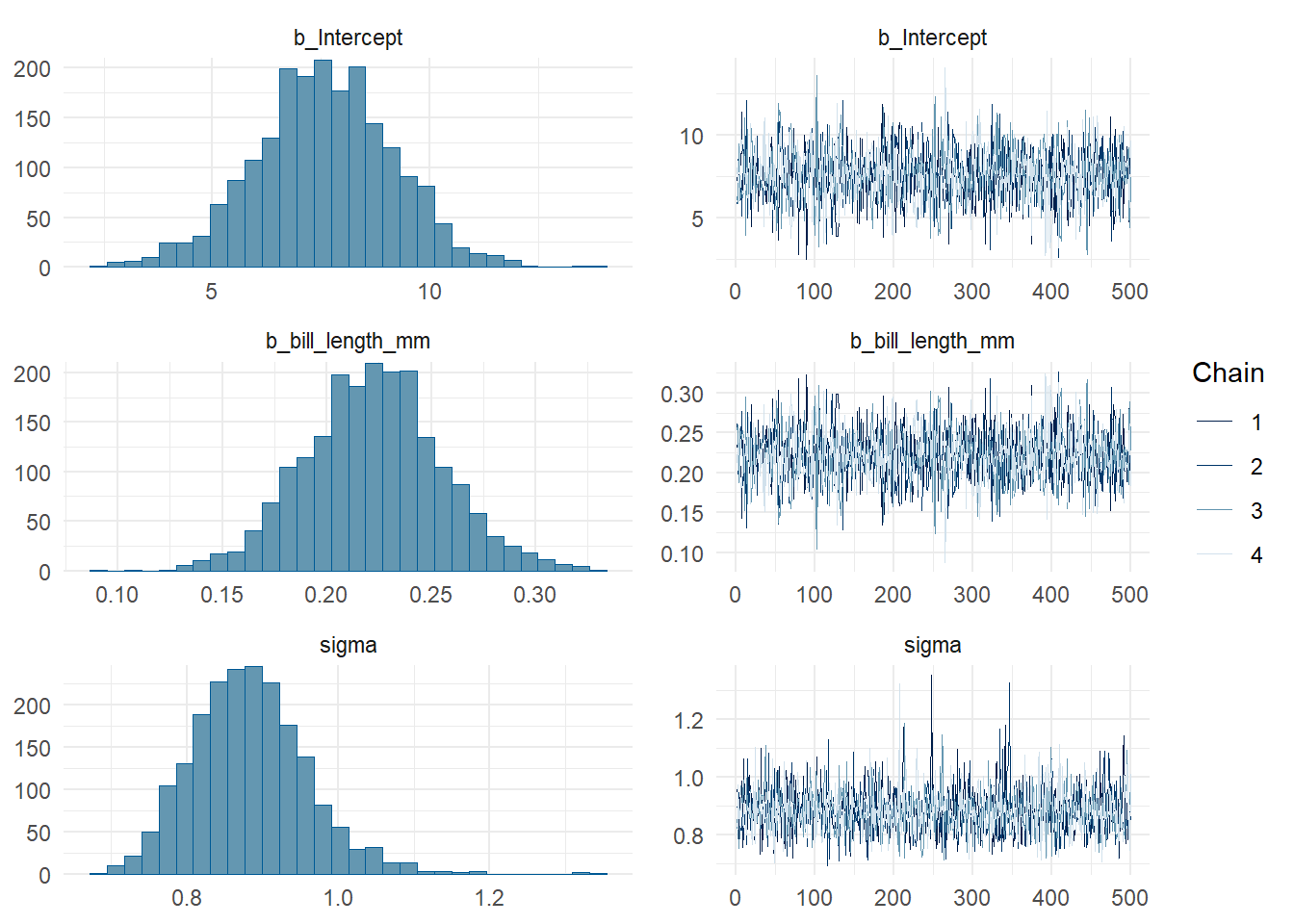
plot(depth_length_brm)

The posterior distribution

This bookdown book is an excellent resource and is the background of these materials.

The posterior distribution gives the likely distributions of the parameters of a model taking into account the prior, the data, and the model structure we defined earlier (in this case a linear model of bill depth as a function of bill length).

MCMC checks

We characterize the posterior by sampling from the posterior using Markov Chain Monte Carlo. MCMC uses “chains” to probabilistically explore the landscape of possible parameter values. MCMC should give us sets of simulated parameter values where more likely values are represented more frequently (proportional to how likely they are). But, after a model runs it is a good idea to check diagnostics on the MCMC procedure to make sure it’s gone smoothly.

summary(depth_length_brm)

 Family: gaussian 
  Links: mu = identity; sigma = identity 
Formula: bill_depth_mm ~ bill_length_mm 
   Data: penguins (Number of observations: 68) 
  Draws: 4 chains, each with iter = 1000; warmup = 500; thin = 1;
         total post-warmup draws = 2000

Regression Coefficients:
               Estimate Est.Error l-95% CI u-95% CI Rhat Bulk_ESS Tail_ESS
Intercept          7.57      1.60     4.29    10.62 1.00     1828     1302
bill_length_mm     0.22      0.03     0.16     0.29 1.00     1803     1301

Further Distributional Parameters:
      Estimate Est.Error l-95% CI u-95% CI Rhat Bulk_ESS Tail_ESS
sigma     0.88      0.08     0.75     1.05 1.00     2180     1472

Draws were sampled using sampling(NUTS). For each parameter, Bulk_ESS
and Tail_ESS are effective sample size measures, and Rhat is the potential
scale reduction factor on split chains (at convergence, Rhat = 1).

Diagnostics:

Trace plots should look like “hairy caterpillars”
Convergence: Rhat should approach 1
ESS should be high (One page I found offers 1000 as a rule of thumb; brms/stan will print a warning about low ESS).

Posterior predictive checks

Here is an excellent blog post on posterior predictive distributions and marginal effects.

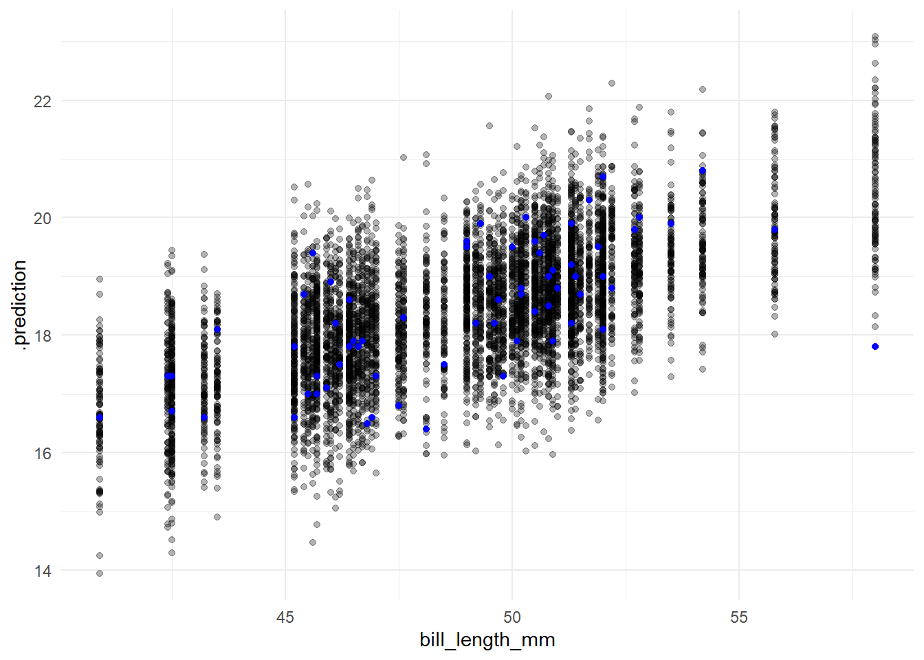
The posterior distribution gives us distributions for the parameters. We want to use these to generate distributions for the data that we would get if we give the original predictor variables to the model. If the model says that the data we observe is highly unlikely - i.e. the posterior predictions are far off from the observed data - we should be suspicious.

The predicted_draws function from the tidybayes package generates posterior predictive distributions. If you provide the original input data as newdata, it will simulate values for the response variable based on the original predictor variables plus the parameters from draws from the posterior.

In this plot, the real data are in blue:

posterior_draws <- tidybayes::predicted_draws(
  depth_length_brm, 
  newdata = penguins,
  ndraws = 100
  )

ggplot(posterior_draws, aes(bill_length_mm, .prediction)) + 
  geom_point(alpha = .3) +
  geom_point(aes(y = bill_depth_mm), color = "blue")